Chapter 1: Understanding Spectral Interpolation

Spectral interpolation is a prevalent technique in data analysis and signal processing, used to estimate values between known data points. While polynomial interpolation is a commonly used method, it often falls short in accuracy. A more effective approach is spectral interpolation, which relies on Fourier transforms. In this article, we will delve into the calculation of spectral interpolating functions and demonstrate how to implement these concepts in Python.

This video, titled "How To Interpolate Data In Python," provides additional insights into interpolation techniques, particularly in the context of Python programming.

Section 1.1: The Basics of Fourier Coefficients

Consider a function ( f ) defined on an equidistant grid.

The Fourier coefficients for the function ( f ) can be expressed as:

Here, ( k ) ranges over ( [-pi/h, pi/h] ). The inverse transform is given by:

To derive the spectral interpolating function, we substitute ( x ) in the above expression. Once we have the interpolating function, we can perform various operations such as differentiation and integration. However, solving the integral directly is not practical for a given ( f ). Instead, we can utilize a clever trick involving the Kronecker delta function.

Section 1.2: The Kronecker Delta Trick

The Kronecker delta is defined as follows:

Substituting this into our initial equation yields the Fourier transform of the Kronecker delta:

For interpolation, we can express it as:

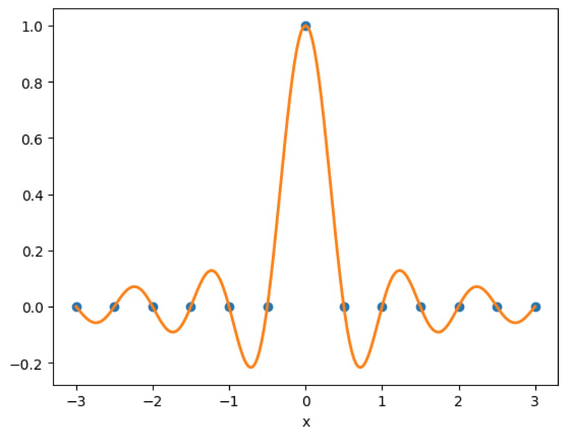
Now, let's visualize this using the sinc function from NumPy. This approach circumvents issues at ( x = 0 ). Note that np.sinc already incorporates a factor of ( pi ) in its argument.

import numpy as np import matplotlib.pyplot as plt

h = 0.5 x_j = np.arange(-3, 3 + h, h) f_j = np.zeros_like(x_j) f_j[abs(x_j) < h / 2] = 1 x = np.linspace(-3, 3, 201) f = np.sinc(x / h) # Note: np.sinc already contains a factor of pi! plt.plot(x_j, f_j, 'o') plt.plot(x, f, lw=2) plt.xlabel('x')

The interpolation may appear excessively wavy, which is a characteristic of the non-smooth Kronecker delta. However, for smoother functions, this method yields significantly better results. A remarkable property of the Kronecker delta is its ability to represent any discrete function in terms of itself:

Since the Fourier transform is linear, we can express our earlier equation as:

After substituting ( x ) for ( x_n ), we derive the interpolating function:

Chapter 2: Implementing Spectral Interpolation in Python

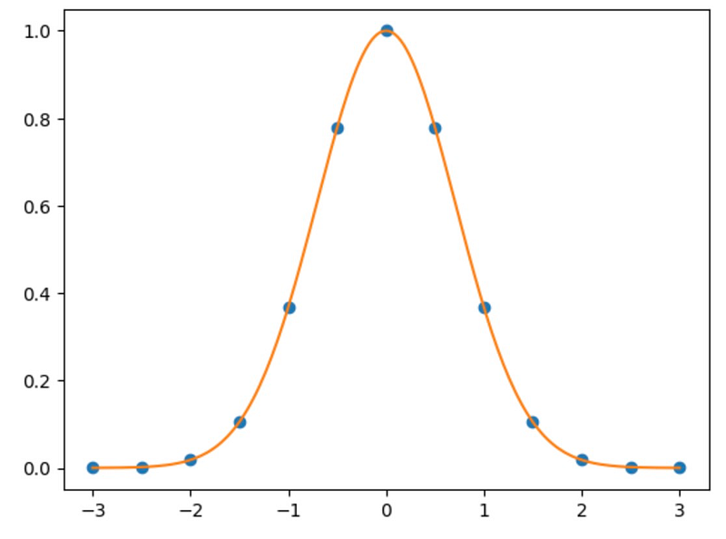
To demonstrate how to implement spectral interpolation, let’s consider a Gaussian function:

def spectral_interpolate(f_j, x_j, x, h):

f = np.zeros_like(x)

for x_n, f_n in zip(x_j, f_j):

f += f_n * np.sinc((x - x_n) / h)

return f

f_j = np.exp(-x_j**2) f = spectral_interpolate(f_j, x_j, x, h) plt.plot(x_j, f_j, 'o') plt.plot(x, f)

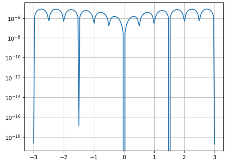
This output appears significantly smoother. To assess the error, we compare it to the exact function we aimed to interpolate:

error = np.abs(np.exp(-x**2) - f) plt.semilogy(x, error) plt.grid()

The observed error is less than ( 10^{-10} ), which is quite impressive given the coarse grid used!

For those interested in further exploring spectral methods, I highly recommend L. Trefethen’s book “Spectral Methods in MATLAB,” which closely aligns with the derivations presented here.

In summary, spectral interpolation serves as a robust technique for estimating values between known data points. The Kronecker delta trick enhances computational efficiency for calculating and implementing spectral interpolating functions.

The second video, "Spectral Analysis in Python (Introduction)," offers a foundational understanding of spectral analysis techniques that complement the methods discussed here.