Mastering Stochastic Integrals: Can We Integrate the Impossible?
Written on
Chapter 1: Introduction to Stochastic Integrals
Stochastic integrals present unique challenges in mathematics. Essentially, you're attempting to integrate a function, denoted as X(t), that exhibits randomness at each moment in time, against another stochastic process, W(t) (often referred to as the Wiener process or Brownian motion).
In a prior discussion, I explored how to determine certain statistical moments of stochastic integrals by leveraging interesting properties of Wiener processes, particularly the Itô isometry, which allows the calculation of the expected value of the square of a stochastic integral. However, what if you wish to compute the integral directly, rather than averaging over multiple outcomes? While numerical methods were employed in my last piece, is that truly the most efficient approach?
To our surprise, there exists a method for analytically evaluating this integral, along with many similar cases. The key is to apply the Itô formula for a function F = f(t, x), which I previously outlined in a different article.

Section 1.1: Applying the Itô Formula
Let's begin by integrating the function according to traditional calculus principles, assuming W²(0) = 0. This seems straightforward, correct? However, applying the Itô formula and differentiating yields some unexpected results.

From the fundamental properties of stochastic integrals, we observe some peculiarities.

The appearance of an extra dt/2 term raises questions about our original integration's completeness. To address this, we can represent this additional term as the differential of a deterministic integral.
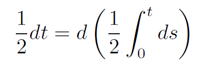
This leads us to an equation that, when both sides are integrated, removes the differential operator. Rearranging reveals the final outcome:

This result adheres to the Itô formula, almost giving the impression of magic. But how can we validate its accuracy?
Chapter 2: Numerical Verification
To test our findings, let’s conduct a numerical experiment. We begin with the Euler-Maruyama approximation:

Here’s the Python code used for implementation:
import numpy as np
import matplotlib.pyplot as plt
# Inputs
t_final = 4
N = 201
t = np.linspace(0, t_final, N)
dt = t[1] - t[0]
# Random samples
N_samples = np.random.normal(loc=0, scale=1, size=N + 1)
W = np.sqrt(dt) * np.cumsum(N_samples[:-1])
dW = np.sqrt(dt) * N_samples[1:]
# Analytic integral
I_analytic = W**2 / 2 - t / 2
# Numerical integral
I_numerical = np.cumsum(W * dW)
# Plot results
plt.figure(1)
plt.plot(t, I_analytic, label="Analytic", color='black')
plt.scatter(t, I_numerical, label="Numeric", color='red')
plt.xlabel('time (s)')
plt.ylabel(r'$int_{0}^{t}W(s)dW(s)$')
plt.legend(frameon=False)
plt.tight_layout()
Executing this multiple times yields results like the following:
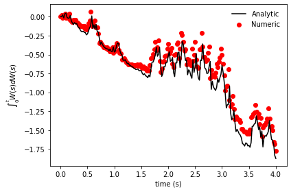
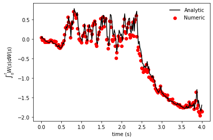
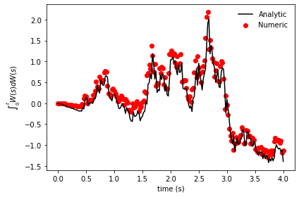
Both the analytical and numerical integrals align quite well. However, a point of confusion may arise regarding the random sample generation. Specifically, why do we take N + 1 samples but slice them differently for W and dW?
# Random samples
N_samples = np.random.normal(loc=0, scale=1, size=N + 1)
W = np.sqrt(dt) * np.cumsum(N_samples[:-1])
dW = np.sqrt(dt) * N_samples[1:]
For W, we use N_samples[:-1] (from the first to second last element), while for dW, we opt for N_samples[1:] (from the second to the last element). This distinction is crucial for achieving convergence in the numerical integral. The Wiener process W(t) is non-anticipating, meaning that we cannot base our steps on future values:
dW(t) = W(t + dt) — W(t)
Instead, we must reference the previous value:
dW(t) = W(t) — W(t — dt)
If we had incorrectly adjusted the code as follows:
# Random samples
N_samples = np.random.normal(loc=0, scale=1, size=N)
W = np.sqrt(dt) * np.cumsum(N_samples[:])
dW = np.sqrt(dt) * N_samples[:]
The outcomes would be markedly different:
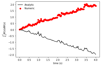
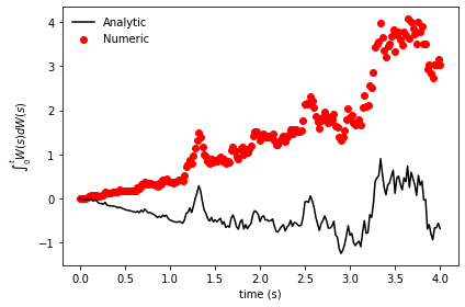
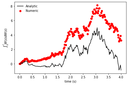
Here, it's evident that the numerical and analytical solutions diverge significantly. The analytical results trend downwards due to the -t/2 term, whereas the numerical results trend upwards due to the mistaken assumption that W(t) is an anticipating process. This subtlety is critical when performing numerical evaluations of stochastic integrals.
Explore the complexities of stochastic calculus in the video titled "Sometimes integration by parts is a bad idea..." - YouTube.
Uncover the challenges of integrals with the video "It 'Cannot' Be Done (Integrals)" - YouTube.